Learn how to use spreadsheets for marketing planning and management

1. Essential Excel. Referencing cells to enter a formula

If you are already a user of Excel, then this section might be superfluous to you, but have a quick read through it, something might pique your interest! For example, do you know why $ cell references are useful or how to concatenate cells to create a URL? They can be handy.

First things first.

As you know, inputting data into a spreadsheet is easy— just click a cell and start typing. However, how do you use formulae in a spreadsheet?

Every cell has its own identification known as a reference: the top bar displays the letters, and the left bar shows the numbers. The combination of Column and letter gives the cell its reference. For example; the first top-left cell is A1 (So: to refer to cells, use the letter first, then the number).

Now you know this, let’s move on to creating your formula. The approach is easy.

• You select a cell – say: Cell C3
• You type the equals symbol (=).
• Then you type your formula: for example: 1+2
• Press Enter

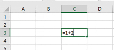
Elementary formula creation.

Voila!

Should you already have data in the cells, say a list of leads generated per day, instead of manually typing in the data, you can refer to the cells the information is in to complete the formula.

• Select the cell you wish the result to be displayed
• Type the equals symbol,
• Either type the cell number or click the respective cell. Note: click one cell, then add the +, then click the cell you wish adding.
• Press Enter

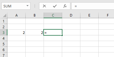
Using cells to calculate.

Can you see what the formula here would be?

It’s =A3+B3. Simple.

When you want to add more numbers, it easiest to use the SUM() function. In this case we can use the formula SUM(A2:B2) in cell C2. The colon is a cell range.

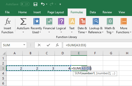
AutoSum function.

Now it’s very likely you picked up these basics very quickly, and if you have, that’s great! For other formulas, try practicing a little more.

Another simple formula:

• To subtract, use the – symbol
• To divide, use the / symbol.
• To multiply, use the * symbol.

Now we move on to a more advanced use of spreadsheets.

Dollar $ cell references

Sometimes, especially when you’re copying and pasting formulas you want to fix the cell so that when it’s pasted to another cell, it’s not updated automatically by Excel which tends to add (or subtract) row and column references when you paste. We find these handiest when creating charts.

For example, if you want to divide multiple cells by a cell, for example, like when calculating a percentage, e.g. here cell A4 contains a percentage based on dividing A2 by E2.

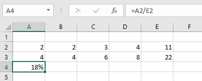
Dividing cell A2 by cell E2

When you copy and paste this formula to B4 – or move it using the black ‘drag handle’ square you will get this error.

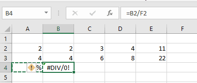
Divide by zero error.

This is because the percentage in B4 is being calculated by dividing through by F2 which doesn’t have a value.

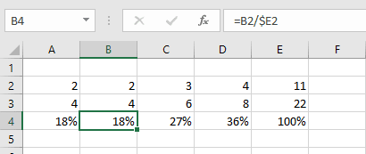
To fix this we add a dollar cell reference $E2 in cell A4 BEFORE we copy and paste it which tells Excel not to change the column when it’s copied.

So now when pasted into cell B the formula stays as =B2/$E2 and the correct answer 18% is displayed.

Using the $-symbol to fix a cell for calculation.

Note that for simplicity it’s often easier to apply the dollar to both column and row reference e.g. =B2/$E$2 then the cell E2 won’t be changed whichever direction it’s moved in.

If you’re scratching your head at this, this is a more advanced topic, which we will cover at the end of this guide, but we wanted to ‘flag it up here’ since you may wonder what these dollars refer to. We cover it again towards the end of this guide with a different example.

Using multiple calculations in one cell.

The input needed for this is quite straightforward. Each calculation is contained within brackets “(“ and “)”. Say,  for example you wish to find out what the average sale is per email sent.

Having a spreadsheet here:

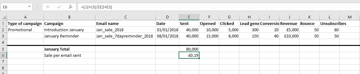
Multiple calculations in one cell.

Your calculation on would be: total sales divided by total emails sent. This translates to: =(J2+J3)/(E2+E3) in the spreadsheet.

In human terms, this simply means:

• First the J2 cell and J3 cell is calculated,
• Then E2 and E3 and calculated,
• Finally, the spreadsheet divides both numbers.

Should you have more calculations, you can ensure they are included in new brackets. For example:

Should you forget the bracket, like so: =(J2+J3)/E2+E3, then it becomes a different story. You’ll say:

• first J2 and J3 are added,
• then divided by E2,
• then E3 is added.

In our example, this results in: £40,000.38 revenue per email. Great result for an email campaign per email, but entirely wrong.

This should highlight the dangers of mistakes in spreadsheets.

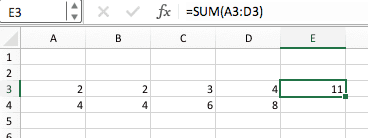
Copying formulas

Of course, you can just copy and paste formulas, but a simple superpower is to use a cell ‘drag handle’ which is the dark square in the bottom right. In this case you would click the black square and using the mouse or track-pad, drag down to copy and paste the formula ‘automagically’ from Cell E3 to E4.

Creating text boxes

Naturally, you won’t just be using spreadsheets for just calculations. Sometimes you need to add text as an explanation or as additional data. You can add text in two ways:

• You add it in a cell:

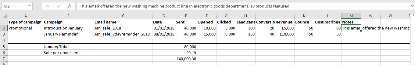
• Or, you can use a text box:
  1. Click insert
  2. Under “Text” click “Text box”
  3. Then just point and click to create a text field
  4. You can use the corners to amend it to your desired shape and location.

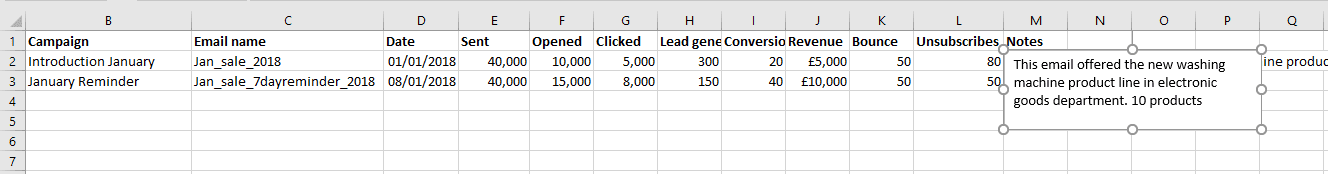
As you can see, the information is placed above the cell, and you can resize it to your will. Conversely, if you wanted your text in a cell formatted to fit the size of the width of the cell, please see Tip 3.

Concatenating strings to form a URL

Concatenation isn’t so easy to say, but it simply means joining together separate strings to form a larger string, or ‘adding text to existing cells’. If you’re wondering, a string is the term by developers to refer to a text variable as compared to a number. There you go, you are a proper geek now!

Concatenation is a very helpful feature to add words or information to existing cells. This function is often used by pay-per-click advertisers to amend their existing keywords.

For example, with pay-per-click ads being displayed depending on a user’s search query, to ensure the maximum reach, PPC professionals would use as many relevant keywords as possible. When they learn of a new keyword to add to their existing list, having the ability to automatically add a new word to their keyword list saves a lot of time.

To join strings or words, use this formula:

1. Select a cell next to the word you wish to amend
2. Type “=” without the parenthesis
3. Select the cell of the word you wish to amend
4. Add & “ keyword” (ensure a space before keyword—INSIDE the quotation marks—else words will be connected.

Example:

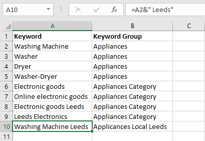
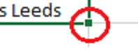
To easily copy it down a list of keywords, select the cell you wish to copy, and drag the little square in the bottom right corner down.

Filters

Sometimes there are so many rows of data, you need some way to restrict it to information in a particular category. The filter-function is simple to use, and very useful when working in spreadsheets.

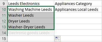
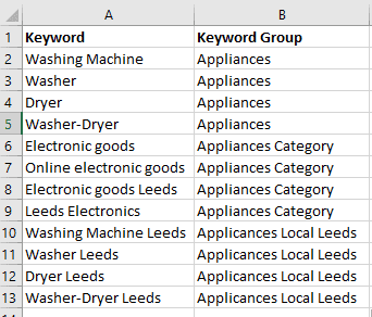
From our previous example, let’s try to change the spreadsheet to only show the keywords for “Appliances Category”.

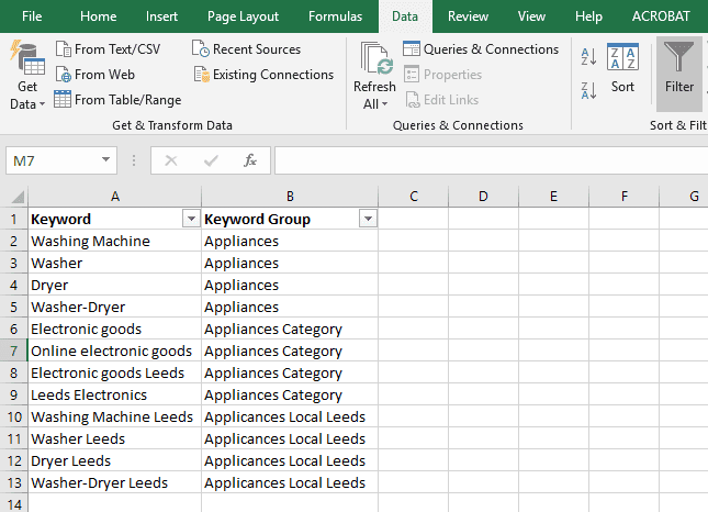
Make sure your data has headers, once you have headers in place:

1. Select row 1,
   • In Excel: Go to “Data” in the menu bar
   • In Google sheets: select Data menu
2. Then:
   • In Excel: select “Filter” by clicking the button on the ‘ribbon’ of functions or choosing ‘Autofilter’ from the menu.
   • In Google sheets: click the “filter views” option, followed by selecting “Create new filter view”

Voila, you have a filter on your data.

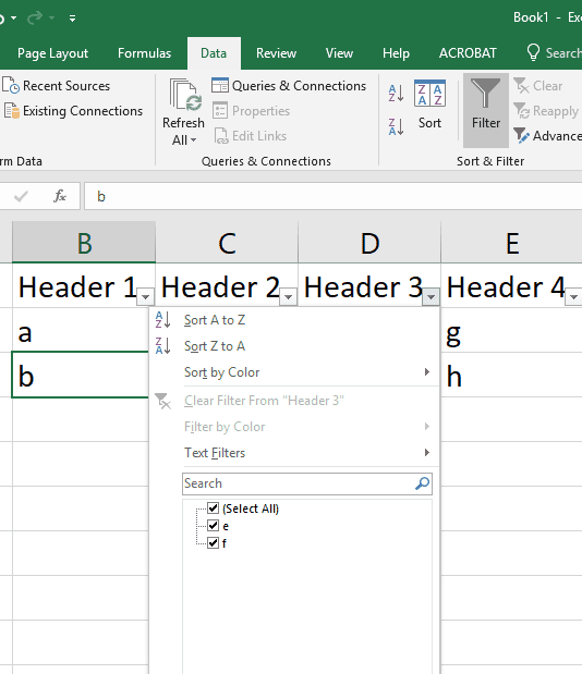
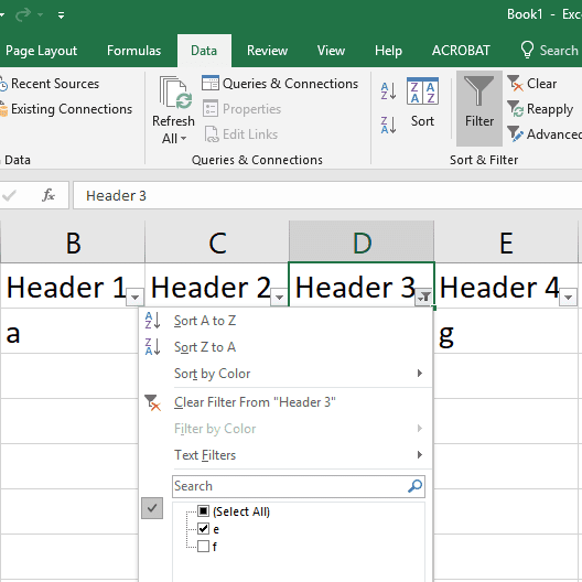
When you select ‘Filter’ or ‘Autofilter’ you will see the header rows of your selection have drop down arrows added. If you click on one of these headers, like below, ‘Header 3’, you can select from all the common strings in your list and when the filter is applied a little funnel is added to the filtered column as shown in the example below.

Filter created

Filter applied

Now you can, for example, click on “Keyword Group” and choose a specific group you wish to view, or amend..

There’s also the ability to filter out certain results. Let’s say you are stopping all “Washer-Dryer” keywords due to discontinuation of the product:

1. Select the Keyword drop down.
   • In Excel: select “Text filter” (it’s classed Number filter with numerical values)
   • In Google sheets: it’s called “Filter by condition”.
2. Then:
   • In Excel: select the option “Does not contains”, and in the dialog box, type the product (e.g. Washer-Dryer).
   • In Google Sheets: select the option” text does not contain” and fill in the text you wish to omit.

Getting sorted

You can also sort your selection of cells alphabetically, or numerically from A-Z or smallest to largest (or vice versa).

Just select the Sort Ascending or Descending option.

This concludes the basic elements of spreadsheets. If you’ve survived so far, well done! We'll be releasing new blog articles throughout the month going through different elements of optimising your spreadsheet use including:

• Advanced formulas and editing
• Formatting cells
• Adjusting views
• Multiple sheet use
• How to work with and clean up raw data
• Pivot tables

Keep coming back to read the whole series and become an excel expert!